Petajisto and Cremers' (2009) ActiveShare and Tracking Error decomposition of money manager returns made what I consider to be revolutionary discoveries, but unfortunately are incredibly costly/difficult to calculate on mutual funds since they require holdings-level data. In his latest two papers, Anders Ekholm demonstrates how to similarly decompose performance armed only with the return stream of the manager. His SelectionShare and TimingShare metrics are both an ingenious standalone contribution and a valuable indirect replication/validation of Petajisto/Cremers. In case my ability to reword/summarize is not sufficient, I'll include the following quote from Ekholm summarizing the research.

"Cremers and Petajisto (2009) and Petajisto (2013) find that past ActiveShare is positively related to future performance. Ekholm (2012) takes a different approach and shows that the excess risk caused by selectivity and timing can be estimated from portfolio returns...

We develop the methodology presented by Ekholm (2012) one step further, and present two new measures that quantify how much selectivity and timing have contributed to total variance. Our SelectionShare and TimingShare measures can be estimated using portfolio returns only, which has both theoretical and practical advantages. Our empirical tests show that all active risk is not equal, as selectivity and timing have opposite effects on performance."

Below with a little replicable R code, I will extend Ekholm's example spreadsheet to a real fund and calculate ActiveAlpha and ActiveBeta (2009 published 2012). Then as Ekholm does, use these ActiveAlpha and ActiveBeta metrics to get SelectionShare and TimingShare (2014). Since these calculations are just basic linear regression, I think it is well within the scope of nearly all readers' abilities.

I am not sure that this will be helpful, and I have not done this in the past, but I will include references to the research within code comments. For someone reading the code and not the content, this will insure that these links do not get lost.

# perform Ekholm (2012,2014) analysis on mutual fund return data

# Ekholm, A.G., 2012
# Portfolio returns and manager activity:
#    How to decompose tracking error into security selection and market timing
# Journal of Empirical Finance, Volume 19, pp 349-€“358

# Ekholm, Anders G., July 21, 2014
# Components of Portfolio Variance:
#    R2, SelectionShare and TimingShare
# Available at SSRN: http://ssrn.com/abstract=2463649

We will, as always, depend on the wonderful and generous contributions of others in the form of R packages. Most of the calculations though are just the base lm(...). I do not think there is any turning back from the pipes in magrittr or pipeR, and since I am addicted I will afford myself the luxury of pipes.

library(quantmod)
library(PerformanceAnalytics)
library(tidyr)
# love me some pipes; will happily translate if pipes aren't your thing
library(pipeR)
#devtools::install_github("ramnathv/rCharts")
library(rCharts)

Get the full set of Fama/French factors from the very generous Kenneth French data library. This example only performs a Jensen regression, so we will only need the Mkt.RF. However, in future installments, we will do the Carhart regression which requires the full factor set. I'll accept full blame for the ugliness in this code.

#daily factors from Kenneth French Data Library
#get Mkt.RF, SMB, HML, and RF
#UMD is in a different file
my.url="http://mba.tuck.dartmouth.edu/pages/faculty/ken.french/ftp/F-F_Research_Data_Factors_daily.zip"
my.tempfile<-paste(tempdir(),"\\frenchfactors.zip",sep="")
paste(tempdir(),"\\F-F_Research_Data_Factors_daily.txt",sep="") %>>%
  (~ download.file( my.url, my.tempfile, method="auto", 
              quiet = FALSE, mode = "wb",cacheOK = TRUE )
  ) %>>%
  (~ unzip(my.tempfile,exdir=tempdir(),junkpath=TRUE ) ) %>>%
  (
    #read space delimited text file extracted from zip
    read.table(file= . ,header = TRUE, sep = "", as.is = TRUE,
                 skip = 4, nrows=23257)
  ) %>>%
  (
    as.xts( ., order.by=as.Date(rownames(.),format="%Y%m%d" ) )
  ) -> french_factors_xts

#now get the momentum factor
my.url="http://mba.tuck.dartmouth.edu/pages/faculty/ken.french/ftp/F-F_Momentum_Factor_daily.zip"
my.usefile<-paste(tempdir(),"\\F-F_Momentum_Factor_daily.txt",sep="")
download.file(my.url, my.tempfile, method="auto", 
              quiet = FALSE, mode = "wb",cacheOK = TRUE)
unzip(my.tempfile,exdir=tempdir(),junkpath=TRUE)
#read space delimited text file extracted from zip
read.table(file=my.usefile, header = TRUE, sep = "",
              as.is = TRUE, skip = 13, nrows=23156) %>>%
  ( #get xts for analysis    
    as.xts( . , order.by=as.Date( rownames(.), format="%Y%m%d"  ) )
  ) %>>%
  #merge UMD (momentum) with other french factors
  ( merge( french_factors_xts, . ) )  %>>%
  na.omit %>>%
  ( .[] / 100 ) %>>%
  (~ plot.zoo(.) ) -> french_factors_xts

getSymbols and Yahoo! Finance is certainly far cheaper than a subscription to CRSP. Since I am in Alabama, I'll choose the largest mutual fund complex in the state Vulcan Value Partners for this example. I am in no way affiliated with Vulcan Value nor should this post in any way be considered a recommendation of the fund. However, for those who would like to know more, Barrons' recently did a profile of Vulcan Waiting to Strike.

#get a fund to analyze
# will use Vulcan Value the biggest mutual fund complex in Alabama
ticker <- 'VVPLX'
ticker %>>% 
  getSymbols( from="1896-01-01", adjust=TRUE, auto.assign=F ) %>>%
  ( .[,4] ) %>>%
  ROC( type = "discrete", n = 1 ) %>>%
  merge ( french_factors_xts ) %>>%
  na.omit -> perfComp

colnames(perfComp)[1] <- gsub( ".Close", "", colnames(perfComp)[1] )

# also subtract risk-free from mutual fund return
perfComp[,1] <- perfComp[,1] - perfComp[,"RF"]

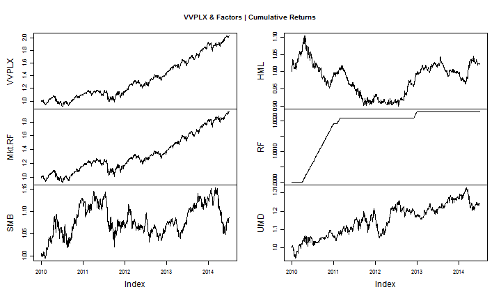
# reasonableness check - plot the fund and factor returns
cumprod(1+perfComp) %>>% plot.zoo ( main = paste0(ticker, " & Factors | Cumulative Returns" ) )

Finally, we can actually calculate Ekholm's SelectionShare and TimingShare. I will try to break it down into simple, easy-to-understand steps.

• Do a Jensen linear regression on fund returns versus the market less risk-free returns.

# do it with lots of comments and no pipes
# to clarify the steps

# 1.  Linear Regression of Fund Return vs (Market - RiskFree)
#      which gives us the well-known Jensen alpha and beta
jensenLM <- lm( data = perfComp, VVPLX ~ Mkt.RF )

• Our linear regression will leave us with some residuals. We will try to explain these residuals by running another linear regression this time on the residuals squared verses the market - riskfree squared.

# 2.  Run another linear regression on the residuals ^2
#       vs the (Mkt - Rf)^2
residuals.df <- data.frame(
  residuals = as.numeric( residuals( jensenLM ) ) ^ 2
  , Mkt.RF_sq = as.numeric( perfComp$Mkt.RF ^ 2 )
)
residualsLM <- lm(
  data = residuals.df
  , residuals.df$residuals ~ residuals.df$Mkt.RF_sq
)

• ActiveAlpha and ActiveBeta will be the square root of the coefficients from the second linear regression.

# 3. Get ActiveAlpha and ActiveBeta from coefficients
#     see
# Ekholm, A.G., 2012
# Portfolio returns and manager activity:
#    How to decompose tracking error into security selection and market timing
# Journal of Empirical Finance, Volume 19, pp 349-€“358
activeAlpha = coefficients( residualsLM )[1] ^ (1/2)
activeBeta = coefficients( residualsLM )[2] ^ (1/2)

• We now have all we need to calculate SelectionShare and TimingShare (see equations 10 and 11 in the paper for a full discussion).

# 4. Last step to calculate SelectionShare and TimingShare
selectionShare = as.numeric(activeAlpha ^ 2 /
                    (
                      var( perfComp$VVPLX ) *
                      (nrow( perfComp ) - 1) / nrow( perfComp )
                    )
                  )

timingShare = as.numeric( activeBeta ^ 2 *
                mean( residuals.df$Mkt.RF_sq ) /
                (
                  var( perfComp$VVPLX ) *
                    ( nrow( perfComp ) - 1) / nrow( perfComp )
                )
              )

We have accomplished our mission. To check that we have not messed up, we can verify the identity (equation 12) and make sure that r^2 + SelectionShare + TimingShare = 1. In effect, this says we have now fully explained the fund returns.

# check our work r^2  + selectionShare + timingShare should equal 1
summary(jensenLM)$"r.squared" + selectionShare + timingShare

[1] 1

I expect to use this Ekholm decomposition a lot, and I hope you will too. To make it easier, I'll make a simple function that will allow us to do the calculations in one-line and also do rolling decompositions.

# return a list with
# 1. a data.frame of ActiveAlpha, ActiveBeta, SelectionShare, and TimingShare
# 2. the first linear regression
jensen_ekholm <- function( data, ticker = NULL ){

  if(is.null(ticker)) ticker <- colnames(data)[1]

  # subtract risk free from manager return
  # not sure if better to assume already done or not
  data[,ticker] <- data[,ticker] - data[,"RF"]

  as.formula ( paste0(ticker, " ~  Mkt.RF" ) ) %>>%
    ( lm( data = data, . ) -> jensenLM )

  jensenLM %>>%
    residuals %>>%
    (. ^ 2 ) %>>%
    (
      data.frame(
        data
        , "fitted_sq" = .
        , lapply(data[,2],function(x){
          structure(
            data.frame( as.numeric(x) ^ 2 )
            , names = paste0(names(x),"_sq")
          ) %>>%
            return
        }) %>>% ( do.call( cbind, . ) )
      ) -> return_data_jensen
    )

  return_data_jensen %>>%
    ( lm( fitted_sq ~ Mkt.RF_sq, data = . ) )%>>%
    coefficients %>>%
    ( . ^ (1/2) ) %>>%
    t %>>%
    (
      structure(
        data.frame(.),
        names = c("ActiveAlpha", paste0("ActiveBeta_",colnames(.)[-1]))
      )
    ) %>>% 
    (
      data.frame(
        .
        , "SelectionShare" = .$ActiveAlpha ^ 2 / (var(return_data_jensen[,ticker]) * (nrow(return_data_jensen) - 1) / nrow(return_data_jensen))
        , "TimingShare" = .$ActiveBeta_Mkt.RF_sq ^ 2* mean( return_data_jensen$Mkt.RF_sq ) / (var(return_data_jensen[,ticker]) * (nrow(return_data_jensen) - 1) / nrow(return_data_jensen))
      )
    ) %>>%
    (
      list( "ekholm" = ., "linmod" = jensenLM )
    ) %>>%
    return
}

We should probably check that our new function generates the same result as our previous calculations.

#add back risk free since function will subtract risk-free
perfComp[,1] <- perfComp[,1] + perfComp[,"RF"]

jensen_ekholm( perfComp ) -> jE

jE$ekholm$SelectionShare ==  selectionShare %>>%
  (~cat(c(
    "<p style='color:", ifelse(.,"green","red"), ";font-size:70%'>Does "
    ,jE$ekholm$SelectionShare
    , " == "
    , selectionShare
    ,"?</p>"
  ))) %>>% as.character

Does 0.0642760267657398 == 0.0642760267657398 ?

jE$ekholm$TimingShare ==  timingShare %>>%
  (~cat(c(
    "<p style='color:", ifelse(.,"green","red"), ";font-size:70%'>Does "
    ,jE$ekholm$TimingShare
    , " == "
    , timingShare
    ,"?</p>"
  ))) %>>% as.character

Does 0.0015160232454823 == 0.0015160232454823 ?

#as another check, this should equal 1
#jE %>>% ( summary(.$linmod)$"r.squared" + jE$ekholm[1,3] + jE$ekholm[1,4] )

In finance, it is almost always more fun and instructive to do functions on a rolling basis. A rolling Ekholm decomposition is easy now with our new function jensen_ekholm.

perfComp %>>%
  rollapply (
    FUN= function(x){
      x %>>%
        jensen_ekholm %>>% 
        ( data.frame( summary(.[["linmod"]])$"r.squared" , .$ekholm ) )  %>>%
        xts(order.by=tail(index(x),1)) -> return_df
      colnames(return_df)[1] <- "R_sq"
      return(return_df)
    }
    , width = 500
    #, by = 100
    , by.column=F
    , fill = NULL
  ) %>>%
  na.fill(0) %>>%
  ( data.frame(date=as.numeric(index(.)),.) ) -> rolling_ekholm

  rolling_ekholm[,c(1,2,5,6)] %>>%
    gather(source,value,-date) %>>%
    (nPlot(
      x = "date"
      , y = "value"
      , group = "source"
      , data = .
      , type = "stackedAreaChart"
      , dom = "rollingChart"
    )) %>>%
    (~ .$xAxis(
      tickFormat = "#!function(d){ return d3.time.format('%b %Y')(new Date( d * 24 * 60 * 60 * 1000 ))}!#"
    ) ) %>>%
    (~ .$chart( useInteractiveGuideline = T ) ) %>>%
    ( cat(noquote(.$html())) )

This research is so compelling that there will be a lot more on its way. Just remember for now that in general SelectionShare is good and TimingShare is bad.